Research
Weak Lensing
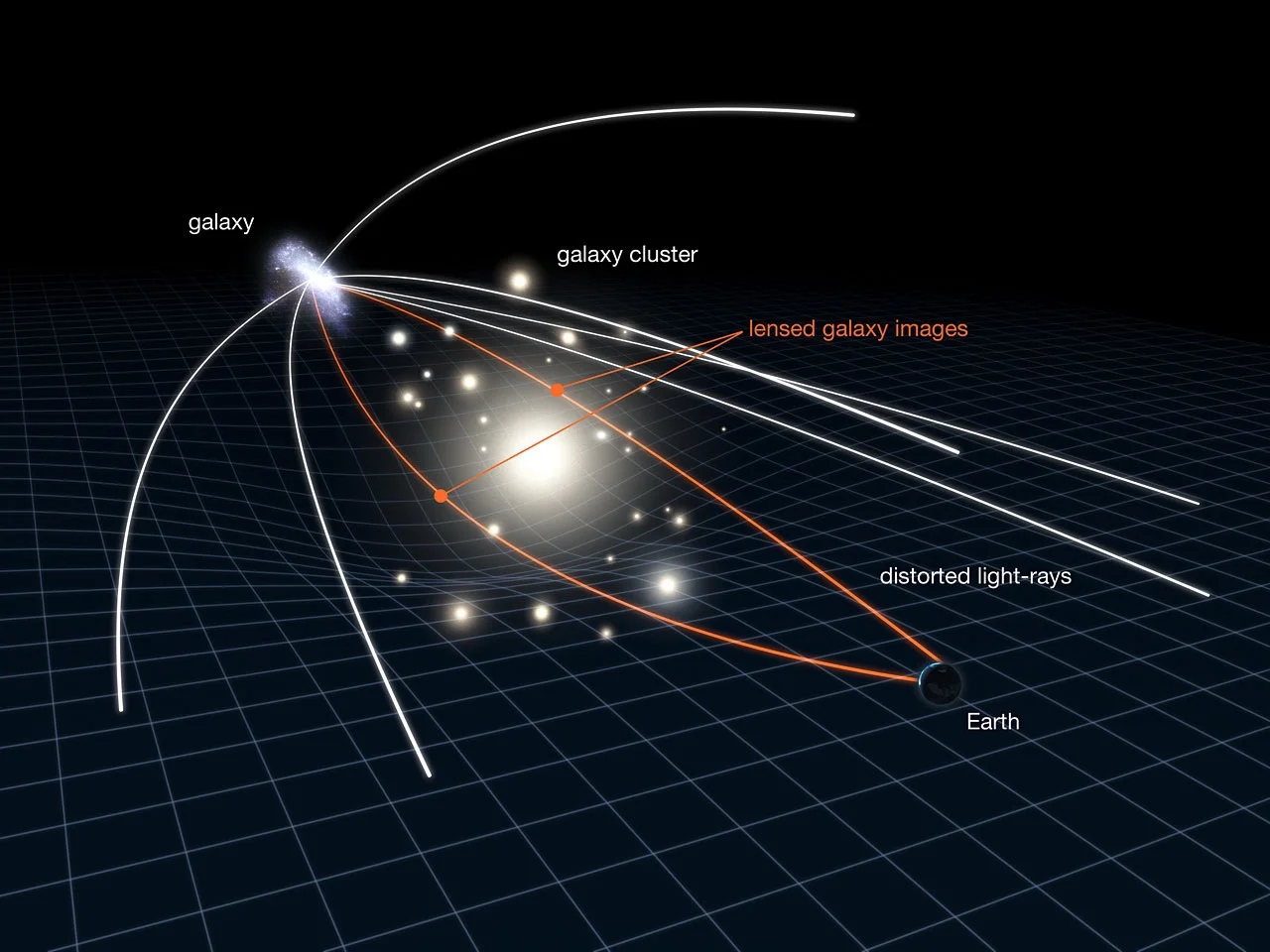
Weak gravitational lensing is the small and coherent change in galaxy shapes caused by matter along the line of sight. From many galaxies we estimate the reduced shear \( g = \gamma/(1-\kappa) \) and reconstruct a convergence map \( \kappa(\theta) \), a projected view of the matter field. The convergence is a weighted line of sight integral of the density contrast \( \delta \):
\[ \kappa(\theta) \;=\; \int_0^{\chi_s} \! \mathrm{d}\chi\; W(\chi)\, \delta\!\big(f_K(\chi)\,\theta,\,\chi\big), \]where \( \chi \) is comoving distance, \( f_K \) is the comoving angular diameter distance, and \( W(\chi) \) is the lensing efficiency.
Two point statistics capture part of the signal, but structure growth makes the field non Gaussian. I summarize extra information with the \( \ell_1 \) norm: at a chosen scale or transform, bin the pixel values and sum absolute values in each bin,
\[ L_1[b] \;=\; \sum_{p:\,x(p)\in b} \lvert x(p)\rvert , \]where \( x(p) \) is the map value used at that step (for example a wavelet coefficient or a smoothed map value). The prediction comes from theory. Using Large Deviation Theory, I build the one point density \( p(x) \) for the same smoothing or transform. The expected content of a bin is then
\[ \mathbb{E}[L_1[b]] \;=\; N_{\mathrm{eff}} \!\int_{x\in b} \lvert x\rvert\, p(x)\,\mathrm{d}x , \]with \( N_{\mathrm{eff}} \) the effective number of pixels after masking and resolution effects.
In practice: reconstruct \( \kappa \) from shear catalogs, choose the analysis scale or wavelet, measure \( L_1[b] \), build \( p(x) \) from Large Deviation Theory, and compare data to theory with an uncertainty model for noise and finite area. This keeps inference close to first principles and light on simulations.
Topological Defects
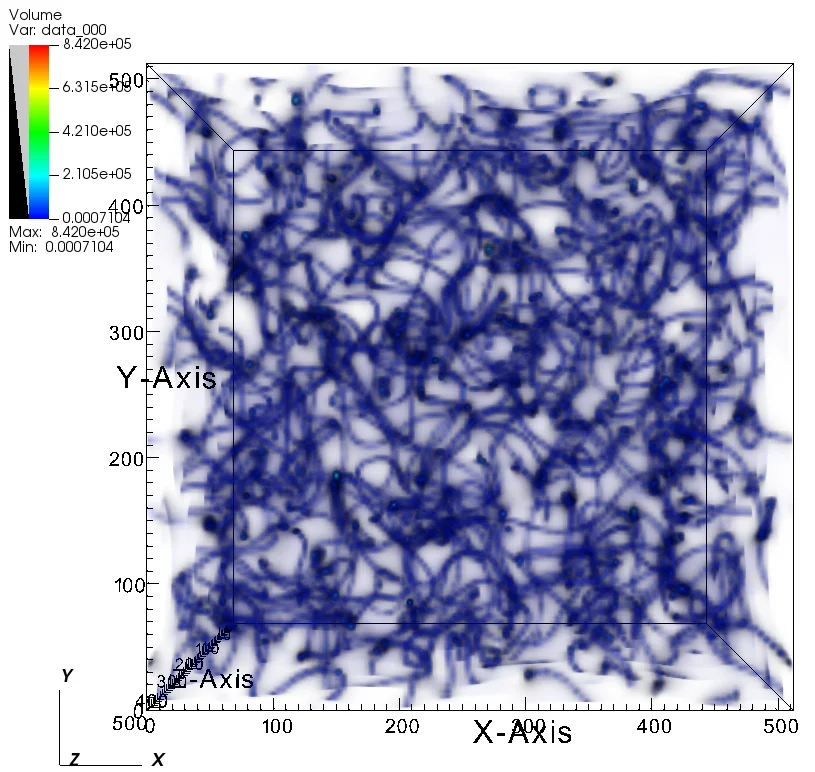
Phase transitions in the early universe can create field configurations that cannot relax away. These are topological defects such as strings, walls, and monopoles. They act as active sources of perturbations: their stress energy keeps sourcing the metric at late times, so the resulting density and velocity fields do not follow the passive evolution of simple initial conditions.
In linear language, defects source scalar, vector, and tensor modes through their stress energy tensor \(T_{\mu\nu}\). Unlike the standard case where vector modes decay, the anisotropic stress of a defect network can maintain vector and tensor contributions with amplitudes that matter for observables. A simple Poisson like statement illustrates the sourcing,
\[ \nabla^2 \Phi \;=\; 4\pi G\,a^2\,\delta\rho_{\mathrm{m}} \;+\; 4\pi G\,a^2\,\delta\rho_{\mathrm{defect}}, \]with additional equations for the divergence free part of the velocity and the tensor modes that include defect anisotropic stress. For strings, a key parameter is the tension \( \mu \) and the dimensionless combination \( G\mu \). Moving strings generate wakes, that is, planar overdensities behind the string, and a web of line like features that bias the late time density field.
The statistics of an evolving network are often described by unequal time correlators of \(T_{\mu\nu}\). In a scaling regime these correlators depend only on ratios of times, which lets us predict how the sourced power moves across scales. The main signatures in large scale structure are additional small scale power, excess vorticity, and non Gaussian features that are not captured by two point summaries alone.
My workflow uses relativistic N body simulations to evolve matter in the presence of a defect source. I implement the source term on the grid, evolve the metric and the particles, and track both scalar and vector contributions. On the analysis side I separate isotropic and anisotropic pieces, measure map based statistics that respond to line like and planar structures, and compare to theory templates that come from the scaling picture and from analytic wake models.
Validation includes controlled tests where I switch off the source to recover the standard case, resolution and volume checks, and sensitivity to the network parameters such as the correlation length, the typical velocity, and \( G\mu \). The goal is a clear link from measurable features in the density and velocity fields back to a small set of physical parameters that describe the network.
Large Deviation Theory
Large Deviation Theory gives a direct way to predict one point statistics in the non linear regime. It starts from simple initial conditions and a spherical collapse mapping, and returns a closed form description of the late time distribution without a large simulation suite.
In practice the inputs are the source redshift distribution, the smoothing or transform that defines the field value, and the variance at that scale. The output is the predicted one point density for that field. From this we obtain the expected content of each value bin for the \( \ell_1 \) norm, which is then compared to measurements with an uncertainty model for noise and finite area.
LDT is fast and transparent, which makes it useful for scans and sensitivity checks. It agrees with perturbation theory in the small variance limit and remains stable deeper into the mildly non linear regime. The main caveats are very small scales where shell crossing, baryons, and intrinsic alignment can matter, and survey systematics that must be tested with mocks.